How my real-time simulations are developed
Quantization in time and 'amplitude'
Time depending processes normally deal with the course
of analogue values with the elapsed time, - a continuous process in time.
Digital devices, like microprocessors, microcontrollers and digital circuits,
are working stepwise in time and in 'variable values' , that means they exhibit
a stepwise quantization of values. The quantization in time is determined e.g.
for micro processors by the processor cycle time, - generally for digital
systems by the 'cycle time'. As you know from your computer that the accuracy
of the values depends on the bit-width of the value ( 8 Bit, 16 Bit, 32 Bit and
higher) you also know that the rate of computation mounts with the processor
cycle frequency. This is the basis of all numerical approaches for time
dependent analogue processes by means of digital technique. It is clear that a
stepwise 'treatment' of the steadily running time can only be accurate enough,
when the cycle time is very short in comparison to the whole time ('eigenzeit')
that the process takes. The Shannon-Theorem tells us as a rule that the cycle
frequency should be at minimum 10 times higher than the 'fastest frequency' of
the process.
Developing the simulation:
| real process: some
'potential variables are running as a function of time. the process could be
observed experimental or you know by experience how it is working |
| - |
| make a model, how the process
works |
| develop a balance equation for the
regarded variables (e.g. temeperature, pressure, force, distance, material
balance ---> |
this leads in most cases to the form of a
differential equation in time:
dy/dt = f(y) |
| - |
| apply the logistic equation method: dy/dt
replaced by the difference quotient for 'slice times' << 'process
time' |
| - |
| develop a program with cyclic structure
in time, e.g. by using in HP VEE an 'on cycle node' |
| - |
| visualize or store data |
The logistic equation method.
The logistic equation method is the reverse method of
the transition to the differential quotient starting from the difference
quotient in mathematics, - that means we go back from the infinitesimal value
dt = 0 to the very small value 'delta t' not equal 0, but small in comparison
to the 'eigenzeit' , i.e. the difference quotient. Let us take a simple example
from chemistry: the kinetic equation of a simple first order reaction
reads:
dc/dt = k*c
if you substitute the differential quotient
by the difference quotient:
delta(c) / delta (t) = k*c
delta(c) =
k*c*delta(t)
with: delta(c) = cj+1 - c j ,
where j +1 = new time step value and j = value of time step before,
you
get:
cj+1 = cj*(k*delta(t) + 1)
This
algebraic equation is called the logistic equation and for very small timesteps
in comparison to the 'lifetime' of the reaction it is able to produce a pretty
good approach to the steady process. Digital systems are 'born' for this form
of equations, they are working 'by nature' in time- and value- quantization.
This can also be realized when programming: you have to create feed-back loops
(recursions) for variables (remember e.g. of C-code i++ = 1 ). The values get
in(de-)cremented every timestep by a little value. The method of the logistic
equation is described in the book of Manuel Jakubith, Grundoperationen und
chemische Reaktionstechnik (Wiley-CH ). The formulas for first and second order
differential equations from the book read:
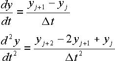
a further example: the accelerated movement
take your browser back for previous text or:
 to main test page